Predict the strength of concrete

📖 Background

Concrete is the most widely used building material in the world. It is a mix of cement and water with gravel and sand. It can also include other materials like fly ash, blast furnace slag, and additives.

The compressive strength of concrete is a function of components and age, the team is testing different combinations of ingredients at different time intervals.

Find a simple way to estimate strength to predict how a particular sample is expected to perform.

The objective is to answer:

1. The average strength of the concrete samples at 1, 7, 14, and 28 days of age.

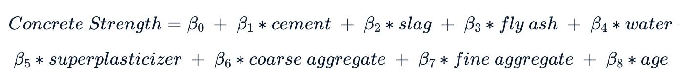
2. The coefficients of regression model using the formula that provided us:

💾 The data

The team has already tested more than a thousand samples (source):

Compressive strength data:

• “cement” - Portland cement in kg/m3

• “slag” - Blast furnace slag in kg/m3

• “fly_ash” - Fly ash in kg/m3

• “water” - Water in liters/m3

• “superplasticizer” - Superplasticizer additive in kg/m3

• “coarse_aggregate” - Coarse aggregate (gravel) in kg/m3

• “fine_aggregate” - Fine aggregate (sand) in kg/m3

• “age” - Age of the sample in days

• “strength” - Concrete compressive strength in megapascals (MPa)

Acknowledgments: I-Cheng Yeh, “Modeling of strength of high-performance concrete using artificial neural networks,” Cement and Concrete Research, Vol. 28, No. 12, pp. 1797-1808 (1998).

Import Libraries

import pandas as pd
import numpy as np
import matplotlib.pyplot as plt
import seaborn as sns
from sklearn.preprocessing import StandardScaler, OrdinalEncoder
from sklearn.model_selection import train_test_split, cross_val_score, KFold
from sklearn.pipeline import Pipeline
from sklearn.linear_model import LinearRegression, LogisticRegression
from sklearn.neighbors import KNeighborsRegressor
from sklearn.tree import DecisionTreeRegressor
from sklearn.ensemble import AdaBoostRegressor, RandomForestRegressor, BaggingRegressor, GradientBoostingRegressor
from sklearn.svm import SVR
from sklearn.model_selection import GridSearchCV
import tensorflow as tf
from sklearn.metrics import mean_squared_error, mean_absolute_error, r2_score
import warnings
warnings.filterwarnings("ignore")

2023-09-07 07:18:16.912242: I tensorflow/tsl/cuda/cudart_stub.cc:28] Could not find cuda drivers on your machine, GPU will not be used.
2023-09-07 07:18:16.963074: I tensorflow/tsl/cuda/cudart_stub.cc:28] Could not find cuda drivers on your machine, GPU will not be used.
2023-09-07 07:18:16.964611: I tensorflow/core/platform/cpu_feature_guard.cc:182] This TensorFlow binary is optimized to use available CPU instructions in performance-critical operations.
To enable the following instructions: AVX2 AVX512F FMA, in other operations, rebuild TensorFlow with the appropriate compiler flags.

2023-09-07 07:18:17.979345: W tensorflow/compiler/tf2tensorrt/utils/py_utils.cc:38] TF-TRT Warning: Could not find TensorRT

Load Data

df = pd.read_csv('data/concrete_data.csv')
df.head()

	cement	slag	fly_ash	water	superplasticizer	coarse_aggregate	fine_aggregate	age	strength
0	540.0	0.0	0.0	162.0	2.5	1040.0	676.0	28	79.986111
1	540.0	0.0	0.0	162.0	2.5	1055.0	676.0	28	61.887366
2	332.5	142.5	0.0	228.0	0.0	932.0	594.0	270	40.269535
3	332.5	142.5	0.0	228.0	0.0	932.0	594.0	365	41.052780
4	198.6	132.4	0.0	192.0	0.0	978.4	825.5	360	44.296075

Data Preprocessing

Data Size and Structure

• Dataset comprises of 1030 observations.

• 8 features and 1 target variable strength.

• All columns are numerical

• No null values

print(f'Shape: {df.shape} \n')
df.info()

Shape: (1030, 9) 

<class 'pandas.core.frame.DataFrame'>
RangeIndex: 1030 entries, 0 to 1029
Data columns (total 9 columns):
 #   Column            Non-Null Count  Dtype  
---  ------            --------------  -----  
 0   cement            1030 non-null   float64
 1   slag              1030 non-null   float64
 2   fly_ash           1030 non-null   float64
 3   water             1030 non-null   float64
 4   superplasticizer  1030 non-null   float64
 5   coarse_aggregate  1030 non-null   float64
 6   fine_aggregate    1030 non-null   float64
 7   age               1030 non-null   int64  
 8   strength          1030 non-null   float64
dtypes: float64(8), int64(1)
memory usage: 72.5 KB

Duplicated Data

A small 2.43% of the dataset are duplicated. I decided to drop these, so now the dataset has 1005 observations.

dup_perc = df.duplicated().sum() / len(df) * 100
print(f'Duplicated percentage: {np.round(dup_perc, 2)}%')
df.drop_duplicates(inplace=True)
print(f'df shape after removing duplicates: {df.shape}')

Duplicated percentage: 2.43%
df shape after removing duplicates: (1005, 9)

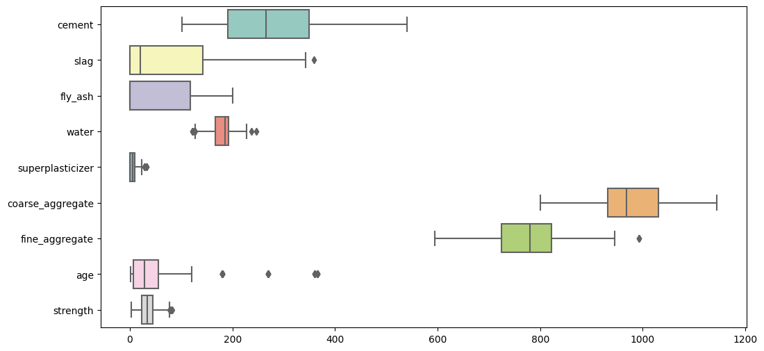
Outliers

Boxplots show that there are outliers in our data, but not many. We will be replacing these outliers with their median.

plt.figure(figsize=(12,6))
sns.boxplot(data=df, orient="h", palette="Set3")
plt.show()

for col_name in df.columns[:-1]:
    q1 = df[col_name].quantile(0.25)
    q3 = df[col_name].quantile(0.75)
    iqr = q3 - q1
    low = q1 - 1.5 * iqr
    high = q3 + 1.5 * iqr
    df.loc[(df[col_name] < low) | (df[col_name] > high), col_name] = df[col_name].median()

Summary Statistics

Variance, skew, and kurtosis is also included.
We can see that all variables have skew are in asymmetric form.

desc = df.describe().T
desc['var'] = df.var(axis=0)
desc['skew'] = df.skew(axis=0)
desc['kurtosis'] = df.kurtosis(axis=0)
desc

	count	mean	std	min	25%	50%	75%	max	var	skew	kurtosis
cement	1005.0	278.629055	104.345003	102.000000	190.680000	265.000000	349.00000	540.000000	10887.879601	0.564997	-0.432463
slag	1005.0	71.367711	85.239740	0.000000	0.000000	20.000000	141.30000	342.100000	7265.813343	0.830465	-0.524116
fly_ash	1005.0	55.535075	64.207448	0.000000	0.000000	0.000000	118.27000	200.100000	4122.596436	0.497324	-1.366457
water	1005.0	182.521294	20.114500	127.300000	168.000000	185.700000	192.00000	228.000000	404.593097	0.126521	-0.076357
superplasticizer	1005.0	5.791846	5.396851	0.000000	0.000000	6.100000	9.90000	23.400000	29.126001	0.514240	-0.312220
coarse_aggregate	1005.0	974.376468	77.579534	801.000000	932.000000	968.000000	1031.00000	1145.000000	6018.584052	-0.065242	-0.583034
fine_aggregate	1005.0	771.628905	78.821267	594.000000	724.300000	780.000000	822.00000	945.000000	6212.792066	-0.335220	-0.198316
age	1005.0	32.117413	27.665333	1.000000	7.000000	28.000000	28.00000	120.000000	765.370663	1.312008	0.876534
strength	1005.0	35.250273	16.284808	2.331808	23.523542	33.798114	44.86834	82.599225	265.194960	0.395653	-0.305402

Exploratory Data Analysis

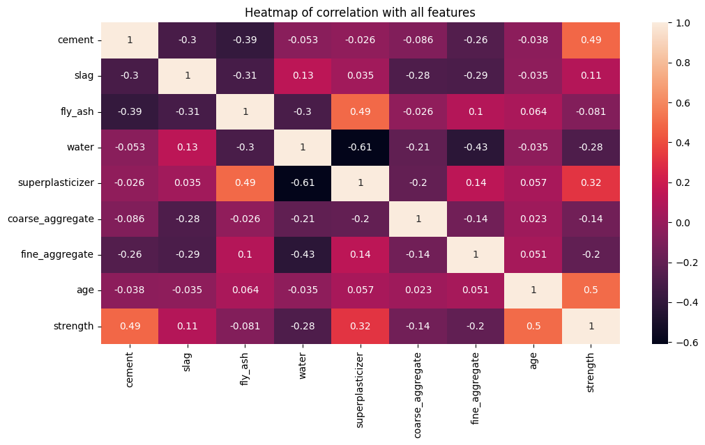
Correlation matrix

Let’s look at the relationship between all the variables and their correlation.
From the heatmap, we observe target variable strength has a high positive correlation cement 0.49, superplasticizer 0.32, and age 0.5.
There is a strong negative correlation (-0.61) between superplasticizer and water.

plt.figure(figsize=(12,6))
sns.heatmap(df.corr(), annot=True)
plt.title('Heatmap of correlation with all features')
plt.show()

Age

Age is a very important characteristic that affects concrete strength.

plt.figure(figsize=(12,6))
sns.countplot(x='age', data=df)
plt.title(label="Count of ages of concrete")
plt.xlabel("Age (Days)")
plt.show()

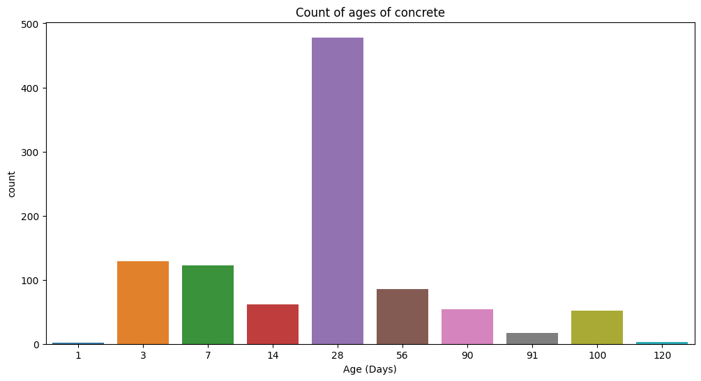
This bar plot shows that age is a categorical variable with a high number of observations at 28 days.
The 28 days time frame is significant because this is the period for concrete to reach 99% of it’s strength. While the concrete continuous to gain strength after that period, the rate of gain is much less compared to that in 28 days.

avg_str_by_day = df.groupby('age').agg(['mean', 'count'])['strength']
avg_str_by_day.reset_index(inplace=True)
avg_str_by_day.age = avg_str_by_day.age.astype(int)
avg_str_by_day = avg_str_by_day.style.set_caption("Average concrete strength at different ages (Days):")
print(f'Average concrete strength: {df.strength.mean()} \n')
avg_str_by_day

Average concrete strength: 35.25027287623584 

Average concrete strength at different ages (Days):

	age	mean	count
0	1	9.452716	2
1	3	18.378023	129
2	7	25.181843	122
3	14	28.751038	62
4	28	37.383788	478
5	56	50.715152	86
6	90	40.480809	54
7	91	68.674649	17
8	100	47.668780	52
9	120	39.647168	3

From the table we can see that average concrete strength at 28 days is similar to the average strength of the entire dataset.

plt.figure(figsize=(12,6))
sns.boxplot(x='age', y='strength', data=df);
plt.title(label="Boxplot of concrete strength at different ages")   
plt.xlabel("Age (Days)")
plt.ylabel("Strength")
plt.show()

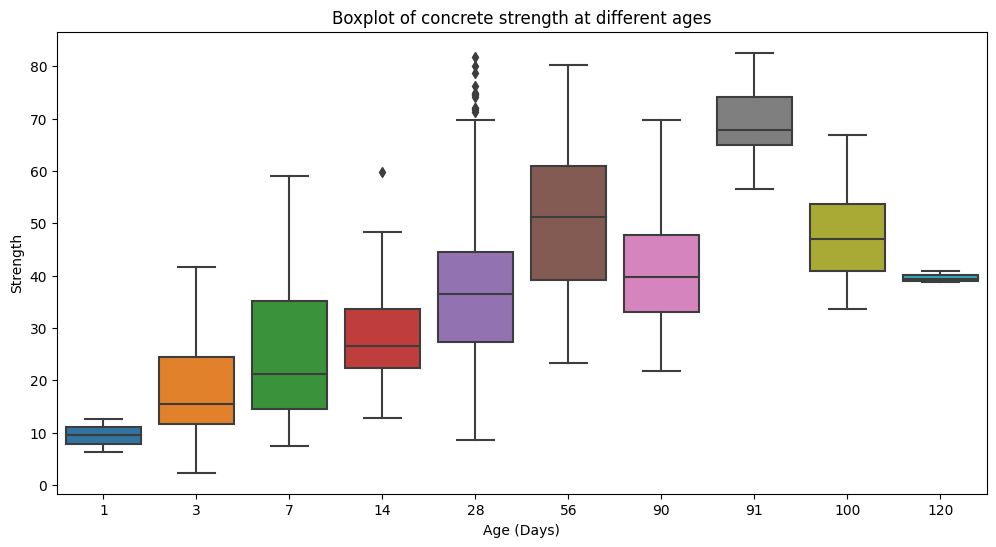
In this boxplot, concrete strength is the highest at 91 days. They have the highest median strenght with a narrow variation. We can also see that strength has the largest variation at 28 days.

1. Average strength of the concrete samples at 1, 7, 14, and 28 days of age.

Average strength of concrete is the lowest after 1 day and increases significantly after 7 days. Strength continues to increase in MPa after 14 and 28 days.

ages = [1, 7, 14, 28]

for age in ages:
    cond = df.age == age
    avg_str = df[cond].strength.mean().round(2)
    if age == 1:
        print(f'Average strength of the concrete sample is {avg_str} MPa at {age} day.')
    else:
        print(f'Average strength of the concrete sample is {avg_str} MPa at {age} days.')

Average strength of the concrete sample is 9.45 MPa at 1 day.
Average strength of the concrete sample is 25.18 MPa at 7 days.
Average strength of the concrete sample is 28.75 MPa at 14 days.
Average strength of the concrete sample is 37.38 MPa at 28 days.

2. Creating predictive model

Now let’s help our colleages in the engineering department find out the coefficients \(\beta_{0}\), \(\beta_{1}\) … \(\beta_{8}\), to use in the following formula:

Train Test Split

Split the data to train (80%) and test (20%) to estimate the performance of machine learning algorithms when they are used to make predictions on data not used to train the model.

features = ['cement', 'slag', 'fly_ash', 'water', 'superplasticizer', 'coarse_aggregate', 'fine_aggregate', 'age']
X = df[features] # Features
y = df['strength'] # Target

# Train Test Split
X_train, X_test, y_train, y_test = train_test_split(X, y, test_size=0.2, random_state=2022)

print('X train data {}'.format(X_train.shape))
print('y train data {}'.format(y_train.shape))
print('X test data  {}'.format(X_test.shape))
print('y test data  {}'.format(y_test.shape))

X train data (804, 8)
y train data (804,)
X test data  (201, 8)
y test data  (201,)

Encoding age

We observed that age is a variabel comprised of a finite set of discrete values with a ranked ordering between values.

def ordinal_encoding_feature(data, feature):    
    '''Transform selected column with ordinal encoder
    
    INPUTS:
    data: dataframe
    feature: column name
    
    OUTPUT:
    d: dataframe with feature ordinally encoded
    '''  
    d = data.copy()
    encoder = OrdinalEncoder()
    # Reshape because only one column is transformed
    encoder.fit(data[feature].values.reshape(-1,1))
    d[feature]= encoder.transform(data.age.values.reshape(-1,1))
    return d
X_train = X_train.pipe(ordinal_encoding_feature, 'age')
X_test = X_test.pipe(ordinal_encoding_feature, 'age')

Model Selection

We will be using a supervised regression model since the target variable strength is labeled and continuous.
Using k-folds cross validation to estimate and compare the performance of models on out-of-sample data using r2 score. This enables us to identify which model is worth improving upon.
GradientBoostRegressor gives the best results out of models, with the highest r2score of 0.89.

pipelines = []
pipelines.append(('Linear Regression', Pipeline([('scaler', StandardScaler()), ('LR', LinearRegression())])))
pipelines.append(('KNN Regressor', Pipeline([('scaler', StandardScaler()), ('KNNR', KNeighborsRegressor())])))
pipelines.append(('SupportVectorRegressor', Pipeline([('scaler', StandardScaler()), ('SVR', SVR())])))
pipelines.append(('DecisionTreeRegressor', Pipeline([('scaler', StandardScaler()), ('DTR', DecisionTreeRegressor())])))
pipelines.append(('AdaboostRegressor', Pipeline([('scaler', StandardScaler()), ('ABR', AdaBoostRegressor())])))
pipelines.append(('RandomForestRegressor', Pipeline([('scaler', StandardScaler()), ('RBR', RandomForestRegressor())])))
pipelines.append(('BaggingRegressor', Pipeline([('scaler', StandardScaler()), ('BGR', BaggingRegressor())])))
pipelines.append(('GradientBoostRegressor', Pipeline([('scaler', StandardScaler()), ('GBR', GradientBoostingRegressor())])))

# Create empty dataframe to store the results
cv_scores = pd.DataFrame({'Regressor':[], 'R2':[], 'Std':[]})

# Cross-validation score for each pipeline for training data
for ind, val in enumerate(pipelines):
    name, pipeline = val
    kfold = KFold(n_splits=5) 
    score = cross_val_score(pipeline, X_train, y_train, cv=kfold, scoring="r2")
    cv_scores.loc[ind] = [name, score.mean(), score.std()]
cv_scores

	Regressor	R2	Std
0	Linear Regression	0.766578	0.026529
1	KNN Regressor	0.788847	0.023574
2	SupportVectorRegressor	0.702593	0.018576
3	DecisionTreeRegressor	0.803986	0.018346
4	AdaboostRegressor	0.764470	0.013887
5	RandomForestRegressor	0.882420	0.012613
6	BaggingRegressor	0.874642	0.009321
7	GradientBoostRegressor	0.885524	0.011444

Model Tuning

Using Grid Search to tune hyperparameters of Gradient Boosting Regressor.

steps = [('scaler', StandardScaler()), ('GBR', GradientBoostingRegressor())]
pipeline = Pipeline(steps)

param_grid=[{'GBR__n_estimators':[100,500,1000], 
             'GBR__learning_rate': [0.1,0.05,0.02,0.01], 
             'GBR__max_depth':[4,6], 
             'GBR__min_samples_leaf':[3,5,9,17], 
             'GBR__max_features':[1.0,0.3,0.1] }]

#search = GridSearchCV(pipeline, param_grid, cv = 5, scoring = 'r2', n_jobs=-1, verbose=1)
#search.fit(X_train, y_train)
#print(search.best_estimator_) 
#print("R Squared:", search.best_score_)

Now that we have identified the best model, let’s use it to predict on our unseen data X_test.

#best_model = search.best_estimator_

# Let's hardcode the parameters to save time
best_model = Pipeline(steps=[('GBR',
                 GradientBoostingRegressor(learning_rate=0.05, max_depth=6,
                                           max_features=0.3,
                                           min_samples_leaf=17,
                                           n_estimators=1000))])

es = tf.keras.callbacks.EarlyStopping(monitor = 'val_loss', mode='min',patience=5, verbose=1)
best_model.fit(X_train, y_train)

Pipeline(steps=[('GBR',
                 GradientBoostingRegressor(learning_rate=0.05, max_depth=6,
                                           max_features=0.3,
                                           min_samples_leaf=17,
                                           n_estimators=1000))])

In a Jupyter environment, please rerun this cell to show the HTML representation or trust the notebook.
On GitHub, the HTML representation is unable to render, please try loading this page with nbviewer.org.

y_pred = best_model.predict(X_test)

Model Evaluation

Let’s evaluate the model’s performance on the testing data to assess the likely future performance of a model.

print(f'Mean Absolute Error (MAE): {mean_absolute_error(y_test, y_pred)}')
print(f'Mean Squared Error (MSE): {mean_squared_error(y_test, y_pred)}')
print(f'RMSE: {mean_squared_error(y_test, y_pred)**0.5}')
print(f'R2 Score: {r2_score(y_test, y_pred)}')

Mean Absolute Error (MAE): 6.2759229895533535
Mean Squared Error (MSE): 63.96244441213967
RMSE: 7.997652431316309
R2 Score: 0.7505082963525445

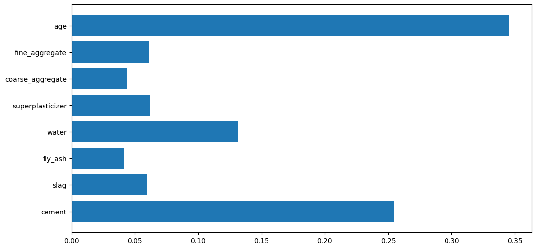
Feature Importance

Using the feature importance of the model, we get the coefficients \(\beta_{0}\), \(\beta_{1}\) … \(\beta_{8}\), to use in the following formula:

betas = best_model[0].feature_importances_
plt.figure(figsize=(12,6))
plt.barh(features, betas)
plt.show()

betas_dict = dict(zip(features, betas))
beta_0 = np.mean(y - np.sum(X*betas, axis=1))
print(f"Concrete Strength = {beta_0} +")
for key in betas_dict.keys():
    if key == "age":
        print(f"{betas_dict[key]} * {key}")
    else:
        print(f"{betas_dict[key]} * {key} +")

Concrete Strength = -167.60301467047782 +
0.25458955256773314 * cement +
0.05994450275185537 * slag +
0.040991604189364705 * fly_ash +
0.13184936195092536 * water +
0.06189292503419931 * superplasticizer +
0.043905713867143197 * coarse_aggregate +
0.06097535136626531 * fine_aggregate +
0.3458509882725137 * age