Inn the Neighborhood - Rental Price Prediction

Project Brief

Inn the Neighborhood is an online platform that allows people to rent out their properties for short stays. Currently, the webpage for renters has a conversion rate of 2%. This means that most people leave the platform without signing up.

The product manager would like to increase this conversion rate. They are interested in developing an application to help people estimate the money they could earn renting out their living space. They hope that this would make people more likely to sign up.

The company has a dataset that includes details about each property rented, as well as the price charged per night. They want to avoid estimating prices that are more than 25 dollars off of the actual price, as this may discourage people.

Objective is to present your findings in two formats:

• Submit a written report summarizing your analysis to your manager. As a data science manager, your manager has a strong technical background and wants to understand what you have done and why.

• Share findings with the product manager in a 10 minute presentation. The product manager has no data science background but is familiar with basic data related terminology.

The data for this analysis can be accessed here: "data/rentals.csv"

The Data

• id: Numeric, the unique identification number of the property

• latitude: Numeric, the latitude of the property

• longitude: Numeric, the longitude of the property

• property_type: Character, the type of property (e.g., apartment, house, etc)

• room_type: Character, the type of room (e.g., private room, entire home, etc)

• bathrooms: Numeric, the number of bathrooms

• bedrooms: Numeric, the number of bedrooms

• minimum_nights: Numeric, the minimum number of nights someone can book

• price: Character, the dollars per night charged

Import Libraries

# Installations
#!pip install geopy lightgbm xgboost verstack --upgrade

import warnings
warnings.filterwarnings('ignore')

import pandas as pd
import numpy as np
import re
from geopy.geocoders import Nominatim
import matplotlib.pyplot as plt
import seaborn as sns
sns.set_style("darkgrid", {"grid.color": ".6", "grid.linestyle": ":"})
from sklearn.preprocessing import OneHotEncoder
from sklearn.compose import make_column_transformer
from sklearn.preprocessing import MinMaxScaler
from sklearn.inspection import permutation_importance
from sklearn.model_selection import train_test_split, cross_val_score, KFold
from verstack import LGBMTuner
from sklearn.feature_selection import SelectFromModel
from sklearn.pipeline import Pipeline
from sklearn.linear_model import LinearRegression, Lasso, LogisticRegression
from sklearn.neighbors import KNeighborsRegressor
from sklearn.svm import SVR
from sklearn.tree import DecisionTreeRegressor
from sklearn.ensemble import AdaBoostRegressor, RandomForestRegressor, BaggingRegressor, GradientBoostingRegressor
from xgboost import XGBRegressor
from lightgbm import LGBMRegressor
from tensorflow.keras.models import Sequential
from tensorflow.keras.layers import Dense, Activation
from tensorflow.keras.optimizers import Adam
from sklearn.metrics import mean_squared_error, mean_absolute_error, r2_score

2023-09-07 07:18:48.527376: I tensorflow/tsl/cuda/cudart_stub.cc:28] Could not find cuda drivers on your machine, GPU will not be used.
2023-09-07 07:18:48.577515: I tensorflow/tsl/cuda/cudart_stub.cc:28] Could not find cuda drivers on your machine, GPU will not be used.
2023-09-07 07:18:48.578600: I tensorflow/core/platform/cpu_feature_guard.cc:182] This TensorFlow binary is optimized to use available CPU instructions in performance-critical operations.
To enable the following instructions: AVX2 AVX512F FMA, in other operations, rebuild TensorFlow with the appropriate compiler flags.

2023-09-07 07:18:49.625065: W tensorflow/compiler/tf2tensorrt/utils/py_utils.cc:38] TF-TRT Warning: Could not find TensorRT

Load the data

rentals_csv = pd.read_csv('data/rentals.csv')
df = rentals_csv.copy()
df.head()

	id	latitude	longitude	property_type	room_type	bathrooms	bedrooms	minimum_nights	price
0	958	37.76931	-122.43386	Apartment	Entire home/apt	1.0	1.0	1	$170.00
1	3850	37.75402	-122.45805	House	Private room	1.0	1.0	1	$99.00
2	5858	37.74511	-122.42102	Apartment	Entire home/apt	1.0	2.0	30	$235.00
3	7918	37.76669	-122.45250	Apartment	Private room	4.0	1.0	32	$65.00
4	8142	37.76487	-122.45183	Apartment	Private room	4.0	1.0	32	$65.00

Data Size and Structure

• Dataset comprises of 8111 observations and 7 characteristics.

• id can be treated as the index

• 7 independent variables: latitude, longitude, property_type, room_type, bathrooms, bedrooms, minimum_nights

  • 5 numerical features, 2 categorical features

• 1 dependent variable: price

• price is treated as object type because of the non-numeric characters in cell, e.g.“$”, “,”.

• 2 variable columns has null/missing values.

df.info()

<class 'pandas.core.frame.DataFrame'>
RangeIndex: 8111 entries, 0 to 8110
Data columns (total 9 columns):
 #   Column          Non-Null Count  Dtype  
---  ------          --------------  -----  
 0   id              8111 non-null   int64  
 1   latitude        8111 non-null   float64
 2   longitude       8111 non-null   float64
 3   property_type   8111 non-null   object 
 4   room_type       8111 non-null   object 
 5   bathrooms       8099 non-null   float64
 6   bedrooms        8107 non-null   float64
 7   minimum_nights  8111 non-null   int64  
 8   price           8111 non-null   object 
dtypes: float64(4), int64(2), object(3)
memory usage: 570.4+ KB

# Set id as index
df.set_index('id', inplace=True)

 def remove_nonnumeric(string):
    """Remove non-numeric characters from string using regex.
    
    INPUTS:
    string - str
    
    OUTPUT
    output - str
    """
    output = re.sub("[^0-9]", "", string)
    return output

# Remove non-numeric characters
df.price = df.price.apply(lambda x: remove_nonnumeric(x))

# Change dtype of price from str to float64 
df.price = df.price.astype('float64') / 100

Summary Statistics

• Features have different scales and units.

• There is a narrow distribution of latitude and longitude values, which suggest the dataset contains properties in the same region.

• There are extreme outliers in minimum_nights, with a max value of 100000000 nights, which would be over 273972 years.

df.describe()

	latitude	longitude	bathrooms	bedrooms	minimum_nights	price
count	8111.000000	8111.000000	8099.000000	8107.000000	8.111000e+03	8111.000000
mean	37.766054	-122.430107	1.395975	1.345874	1.234526e+04	225.407101
std	0.022937	0.026967	0.923213	0.925298	1.110357e+06	412.253039
min	37.704630	-122.513060	0.000000	0.000000	1.000000e+00	0.000000
25%	37.751450	-122.442830	1.000000	1.000000	2.000000e+00	100.000000
50%	37.769150	-122.424650	1.000000	1.000000	4.000000e+00	150.000000
75%	37.785670	-122.410615	1.500000	2.000000	3.000000e+01	240.000000
max	37.828790	-122.368570	14.000000	14.000000	1.000000e+08	10000.000000

# Remove outliers in columns minimum_nights and price using IQR
quant_cols = ["minimum_nights", "price"]

for col_name in quant_cols:
    q1 = df[col_name].quantile(0.25)
    q3 = df[col_name].quantile(0.75)
    iqr = q3 - q1
    low = q1 - 1.5 * iqr
    high = q3 + 1.5 * iqr

    df = df[df[col_name] < high]
    df = df[df[col_name] > low]
df.describe()

	latitude	longitude	bathrooms	bedrooms	minimum_nights	price
count	7389.000000	7389.000000	7377.000000	7386.000000	7389.000000	7389.000000
mean	37.765445	-122.430049	1.339637	1.225968	15.288131	162.706320
std	0.023001	0.027253	0.906060	0.792813	14.291618	87.043561
min	37.704630	-122.513060	0.000000	0.000000	1.000000	0.000000
25%	37.750730	-122.442950	1.000000	1.000000	2.000000	98.000000
50%	37.768500	-122.424370	1.000000	1.000000	5.000000	148.000000
75%	37.785220	-122.410380	1.500000	2.000000	30.000000	208.000000
max	37.828790	-122.368570	14.000000	14.000000	70.000000	449.000000

Completeness of Data

• Less than 0.2% of missing values present in columns bathroom and bedrooms

• Since, the missing observations only account for a small amount of the dataset, we can drop these observations.

# Percentage of dataset is null
df.isnull().sum() / len(df) * 100

latitude          0.000000
longitude         0.000000
property_type     0.000000
room_type         0.000000
bathrooms         0.162404
bedrooms          0.040601
minimum_nights    0.000000
price             0.000000
dtype: float64

# Drop null values
df = df.dropna()

Data Cleaning Summary

• Set id as index.

• Removed non-numeric characters from price.

• Dropped extreme outliers in minimum_nights and price.

• Drop rows with null values.

Exploratory Data Analysis

Correlation

• There is a positive correlation between number of bathrooms and bedrooms.

• Price has the highest positive correlation with the number of bedrooms.

• Price has a negative correlation with the number of bathrooms and minimum nights.

• There is no strong correlation between variables.

# Visualizing the correlations between numerical variables
plt.figure(figsize=(10,8))
sns.heatmap(df.corr(), cmap="RdBu", annot=True)
plt.title("Correlations Between Variables", size=15)
plt.show()

---------------------------------------------------------------------------
ValueError                                Traceback (most recent call last)
Cell In[11], line 3
      1 # Visualizing the correlations between numerical variables
      2 plt.figure(figsize=(10,8))
----> 3 sns.heatmap(df.corr(), cmap="RdBu", annot=True)
      4 plt.title("Correlations Between Variables", size=15)
      5 plt.show()

File /opt/hostedtoolcache/Python/3.8.17/x64/lib/python3.8/site-packages/pandas/core/frame.py:10054, in DataFrame.corr(self, method, min_periods, numeric_only)
  10052 cols = data.columns
  10053 idx = cols.copy()
> 10054 mat = data.to_numpy(dtype=float, na_value=np.nan, copy=False)
  10056 if method == "pearson":
  10057     correl = libalgos.nancorr(mat, minp=min_periods)

File /opt/hostedtoolcache/Python/3.8.17/x64/lib/python3.8/site-packages/pandas/core/frame.py:1838, in DataFrame.to_numpy(self, dtype, copy, na_value)
   1836 if dtype is not None:
   1837     dtype = np.dtype(dtype)
-> 1838 result = self._mgr.as_array(dtype=dtype, copy=copy, na_value=na_value)
   1839 if result.dtype is not dtype:
   1840     result = np.array(result, dtype=dtype, copy=False)

File /opt/hostedtoolcache/Python/3.8.17/x64/lib/python3.8/site-packages/pandas/core/internals/managers.py:1732, in BlockManager.as_array(self, dtype, copy, na_value)
   1730         arr.flags.writeable = False
   1731 else:
-> 1732     arr = self._interleave(dtype=dtype, na_value=na_value)
   1733     # The underlying data was copied within _interleave, so no need
   1734     # to further copy if copy=True or setting na_value
   1736 if na_value is not lib.no_default:

File /opt/hostedtoolcache/Python/3.8.17/x64/lib/python3.8/site-packages/pandas/core/internals/managers.py:1794, in BlockManager._interleave(self, dtype, na_value)
   1792     else:
   1793         arr = blk.get_values(dtype)
-> 1794     result[rl.indexer] = arr
   1795     itemmask[rl.indexer] = 1
   1797 if not itemmask.all():

ValueError: could not convert string to float: 'Apartment'

<Figure size 1000x800 with 0 Axes>

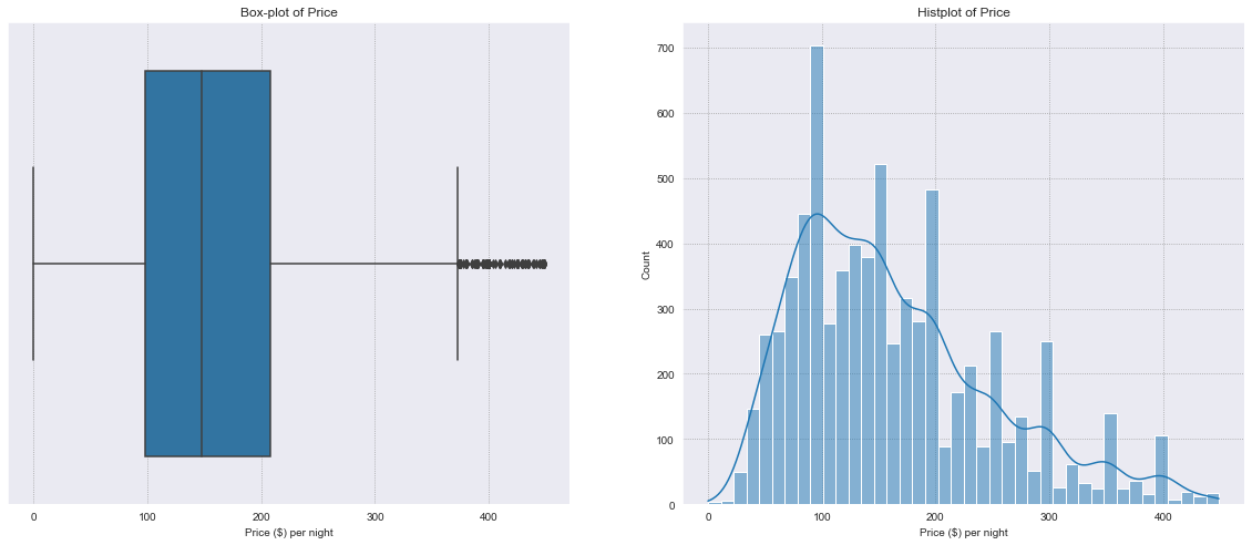
Price

Our target variable price is a continuous numerical variable.
The distribution is right skewed, with most properties costing around $100.00 per night.
Recall that outliers have already been removed from price.

fig, (ax1, ax2) = plt.subplots(1,2, figsize=(20,8))
sns.boxplot(x='price', data=df, ax=ax1)
sns.histplot(x='price', data=df, ax=ax2, kde=True)
ax1.set_title('Box-plot of Price')
ax2.set_title('Histplot of Price')
ax1.set_xlabel('Price ($) per night')
ax2.set_xlabel('Price ($) per night')
plt.show()

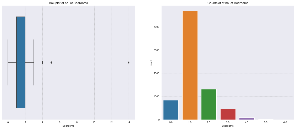
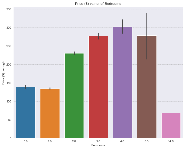
Bedrooms

bedrooms is a discrete numerical variable. It has the highest positive correlation with price.
The distribution is right skewed, with most properties having 1 bathroom. Different variability of the price is present for each number of bedrooms.

fig, (ax1, ax2) = plt.subplots(1,2, figsize=(20,8))
sns.boxplot(x='bedrooms', data=df, ax=ax1)
sns.countplot(x='bedrooms', data=df, ax=ax2)
ax1.set_title('Box-plot of no. of Bedrooms')
ax2.set_title('Countplot of no. of Bedrooms')
ax1.set_xlabel('Bedrooms')
ax2.set_xlabel('Bedrooms')
plt.show()

# Price corresponding to no. of Bedrooms
plt.figure(figsize=(10,8))
ax = sns.barplot(y='price', x='bedrooms', data=df)
ax.set_title('Price ($) vs no. of Bedrooms')
ax.set_xlabel('Bedrooms')
ax.set_ylabel('Price ($) per night')
plt.show()

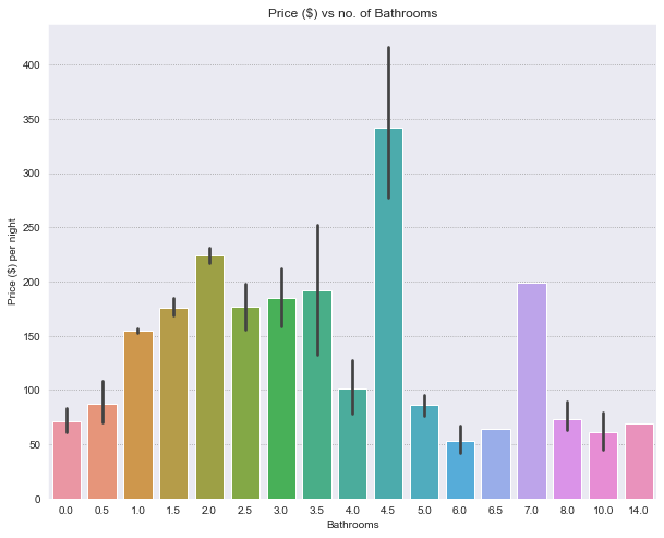
Bathrooms

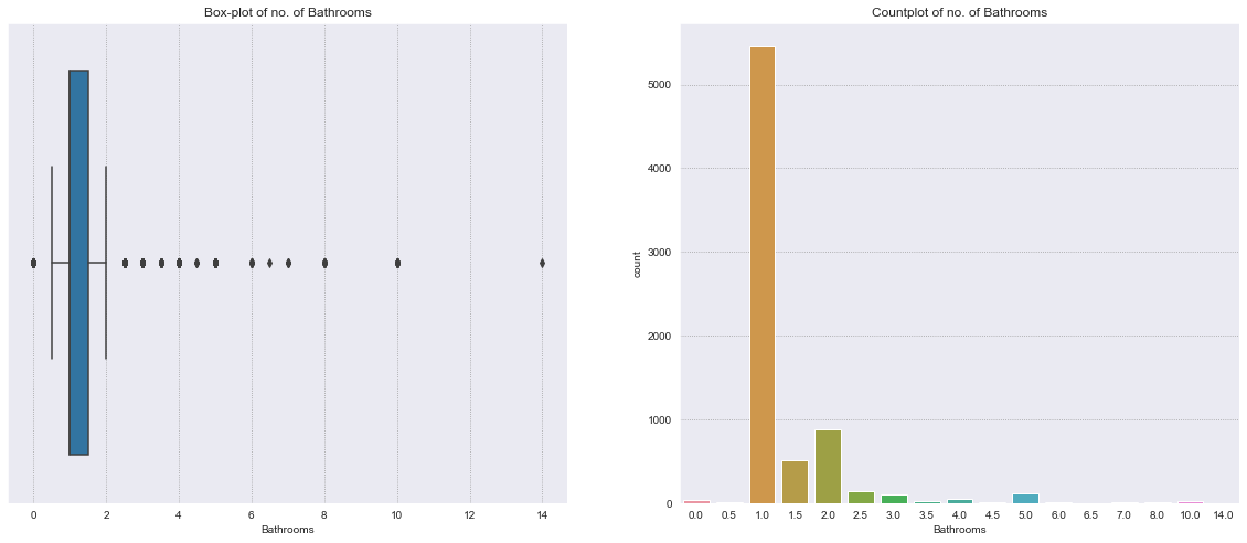
bathrooms is a discrete numerical variable. It has a weak positive correlation with bedrooms.
Contextual information: A full bathroom has a sink, toilet, and either a tub/shower combo or separate tub and shower. Whereas, a half-bath has a sink and a toilet - no tub or shower.
The distribution is right skewed, with most properties having 1 bathroom. Different variability of the price is present for each number of bathrooms.

fig, (ax1, ax2) = plt.subplots(1,2, figsize=(20,8))
sns.boxplot(x='bathrooms', data=df, ax=ax1)
sns.countplot(x='bathrooms', data=df, ax=ax2)
ax1.set_title('Box-plot of no. of Bathrooms')
ax2.set_title('Countplot of no. of Bathrooms')
ax1.set_xlabel('Bathrooms')
ax2.set_xlabel('Bathrooms')
plt.show()

# Price corresponding to no. of Bathrooms
plt.figure(figsize=(10,8))
ax = sns.barplot(y='price', x='bathrooms', data=df)
ax.set_title('Price ($) vs no. of Bathrooms')
ax.set_xlabel('Bathrooms')
ax.set_ylabel('Price ($) per night')
plt.show()

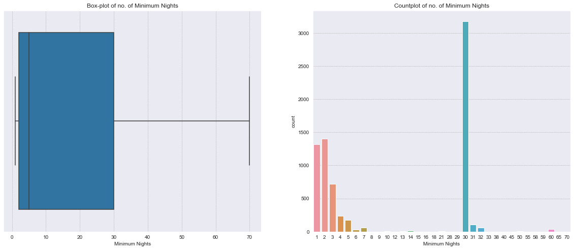
Minimum Nights

minimum_nights is a discrete numerical variable.
The distribution is right skewed and bimodal, with most properties requiring a minimum of 30 or 1-3 nights of stay.
Recall that outliers have already been removed from Minimum Nights.

fig, (ax1, ax2) = plt.subplots(1,2, figsize=(20,8))
sns.boxplot(x='minimum_nights', data=df, ax=ax1)
sns.countplot(x='minimum_nights', data=df, ax=ax2)
ax1.set_title('Box-plot of no. of Minimum Nights')
ax2.set_title('Countplot of no. of Minimum Nights')
ax1.set_xlabel('Minimum Nights')
ax2.set_xlabel('Minimum Nights')
plt.show()

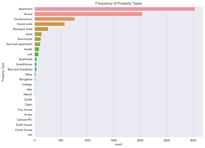
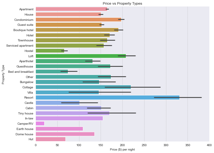
Property Type

property_type is a categorical variable. There are 26 property types.
Most properties are Apartments. The most expensive type being resorts, and the cheapest being Camper/RV.
Different variability of the price is present for each property type. For example, cottages has a wide range of prices, whereas apartments have a narrow range.

print(f"No. of property types: {len(df['property_type'].unique())}")

# Frequency of each property type
plt.figure(figsize=(10,8))
ax = sns.countplot(y='property_type', data=df, order = df['property_type'].value_counts().index)
ax.set_title('Frequency of Property Types')
ax.set_ylabel('Property Type')
plt.show()

No. of property types: 26

# Price of each property type
plt.figure(figsize=(10,8))
ax = sns.barplot(x='price', y='property_type', data=df, order = df['property_type'].value_counts().index)
ax.set_title('Price vs Property Types')
ax.set_ylabel('Property Type')
ax.set_xlabel('Price ($) per night')
plt.show()

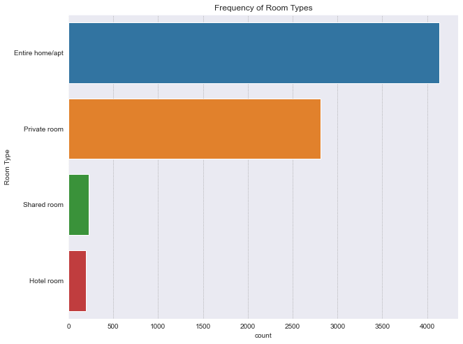
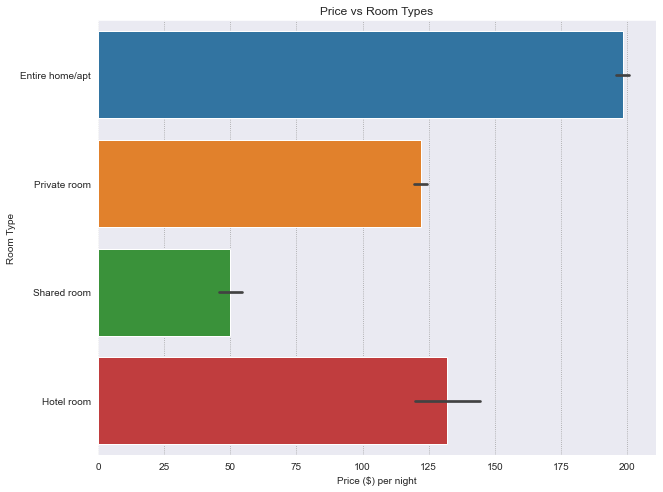
Room Type

room_type is a categorical variable. There are 4 room types.
Most rooms are Entire home/apt. The most expensive type being Entire home/apt, and the cheapest being Shared Room.

print(f"No. of room types: {len(df['room_type'].unique())}")

# Frequency of each room type
plt.figure(figsize=(10,8))
ax = sns.countplot(y='room_type', data=df, order = df['room_type'].value_counts().index)
ax.set_title('Frequency of Room Types')
ax.set_ylabel('Room Type')
plt.show()

No. of room types: 4

# Price of each room type
plt.figure(figsize=(10,8))
ax = sns.barplot(x='price', y='room_type', data=df, order = df['room_type'].value_counts().index)
ax.set_title('Price vs Room Types')
ax.set_ylabel('Room Type')
ax.set_xlabel('Price ($) per night')
plt.show()

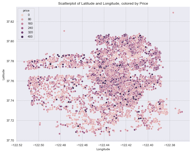
Latitude and Longitude

Properties are located near San Francisco.
Scatterplot does not show distinct price clusters based on latitude and longitude.

# Get address from Latitude and Longitude
geolocator = Nominatim(user_agent="geoapi")
sample_df = df.sample(1)
Latitude, Longitude = sample_df['latitude'].astype(str), sample_df['longitude'].astype(str)
location = geolocator.reverse(Latitude + "," + Longitude)
print(location)

# Visualization of latitude and longitude
plt.figure(figsize=(10,8))
sns.scatterplot(data=df, x='longitude', y='latitude', hue='price')
plt.title('Scatterplot of Latitude and Longitude, colored by Price')
plt.xlabel('Longitude')
plt.ylabel('Latitude')
plt.show()

1449, Baker Street, Western Addition, San Francisco, California, 94115, United States

Train Test Split

Split the data to train (80%) and test (20%) to estimate the performance of machine learning algorithms when they are used to make predictions on data not used to train the model.

X = df.iloc[:, :-1] # Features
y = df['price'] # Target

# Train Test Split
X_train, X_test, y_train, y_test = train_test_split(X, y, test_size=0.2, random_state=2022)

print('X train data {}'.format(X_train.shape))
print('y train data {}'.format(y_train.shape))
print('X test data  {}'.format(X_test.shape))
print('y test data  {}'.format(y_test.shape))

X train data (5899, 7)
y train data (5899,)
X test data  (1475, 7)
y test data  (1475,)

Feature Engineering

Performed after Train Test split to prevent information leakage from the test set.

• Convert categorical variables into a format that can be readily used by machine learning algorithms using One-Hot-Encoding.

• Cartesian coordinates into polar coordinates

• Scale input variables to improve the convergence of algorithms that do not possess the property of scale invariance.

One-Hot-Encoding

# Categorical Features
cat_cols = ['property_type', 'room_type']

# Transformer Object
ohe = make_column_transformer(
    (OneHotEncoder(handle_unknown='ignore'), 
     cat_cols))

def encode(transformer, df):
    """ Apply transformer columns of a pandas DataFrame
    
    INPUTS:
    transformer: transformer object
    df: pandas DataFrame
    
    OUTPUT:
    transformed_df: transformed pandas DataFrame
    
    """
    transformed = transformer.fit_transform(df[cat_cols]).toarray()
    transformed_df = pd.DataFrame(transformed, columns=transformer.get_feature_names())
    return transformed_df

# Apply transformation on both Train and Test set
encoded_train = encode(ohe, X_train)
encoded_train.index = X_train.index
encoded_test = encode(ohe, X_test)
encoded_test.index = X_test.index

print(f"encoded_train shape: {encoded_train.shape}")
print(f"encoded_test shape: {encoded_test.shape}")

# Join encoded cols to Train and Test set, drop original column
X_train = X_train.join(encoded_train)
X_train.drop(cat_cols, axis=1, inplace=True)
X_test = X_test.join(encoded_test)
X_test.drop(cat_cols, axis=1, inplace=True)

# Ensure Train and Test have the same no. of columns
train_cols = list(X_train.columns)
test_cols = list(X_test.columns)
cols_not_in_test = {c:0 for c in train_cols if c not in test_cols}
X_test = X_test.assign(**cols_not_in_test)
cols_not_in_train = {c:0 for c in test_cols if c not in train_cols}
X_train = X_train.assign(**cols_not_in_train)

print(f"X_train shape: {X_train.shape}")
print(f"X_test shape: {X_test.shape}")

encoded_train shape: (5899, 30)
encoded_test shape: (1475, 23)
X_train shape: (5899, 35)
X_test shape: (1475, 35)

Geospaital Features

Transform Cartesian coordinates into polar coordinates.

# Geospatial Features
geo_cols = ['latitude', 'longitude']

def cart2pol(x, y):
    """ Convert cartesian coordinates into polar coordinates
    
    INPUT
    x, y: Cartesian coorindates
    
    OUTPUT
    rho, phi: Polar coordinates
    """
    rho = np.sqrt(x**2 + y**2)
    phi = np.arctan2(y, x)
    return rho, phi

rho, phi = cart2pol(X_train['longitude'], X_train['latitude'])
X_train['rho'] = rho
X_train['phi'] = phi
rho, phi = cart2pol(X_test['longitude'], X_test['latitude'])
X_test['rho'] = rho
X_test['phi'] = phi

print(f"X_train shape: {X_train.shape}")
print(f"X_test shape: {X_test.shape}")

X_train shape: (5899, 37)
X_test shape: (1475, 37)

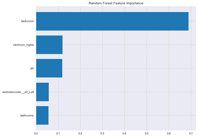
Variable Importance with Random Forest

Using a simple random forest with 100 trees to get a quick overview of the top 5 relative permutation importance for each variable.
According to the random forest, bedrooms is the most important feature. This is expected because it has the highest correlation to the price.

rf = RandomForestRegressor(n_estimators=100, random_state=2022)
rf.fit(X_train, y_train)
perm_importance = permutation_importance(rf, X_test, y_test)

plt.figure(figsize=(10,8))
sorted_idx = perm_importance.importances_mean.argsort()[-5:]
plt.barh(X_train.columns[sorted_idx], perm_importance.importances_mean[sorted_idx])
plt.title("Random Forest Feature Importance")
plt.show()

Feature Selection

Recognize that many new features were generated during feature engineering.
Using Lasso Regularization to identify and select a subset of input variables that are most relevant to the target variable.
Non-important features are removed.

# Lasso Regularization
sel_lasso = SelectFromModel(LogisticRegression(C=1, penalty='l1', solver='liblinear', random_state=2022))
sel_lasso.fit(X_train, y_train)
sel_lasso.get_support()

array([ True,  True,  True,  True,  True,  True,  True,  True,  True,
        True, False, False, False,  True, False, False, False,  True,
        True,  True,  True,  True, False, False,  True,  True,  True,
        True, False,  True, False,  True,  True,  True,  True,  True,
        True])

# make a list with the selected features and print the outputs
selected_feat = X_train.columns[(sel_lasso.get_support())]

print('total features: {}'.format((X_train.shape[1])))
print('selected features: {}'.format(len(selected_feat)))
print('features with coefficients shrank to zero: {}'.format(np.sum(sel_lasso.estimator_.coef_ == 0)))

total features: 37
selected features: 27
features with coefficients shrank to zero: 10531

X_train = X_train[selected_feat]
X_test = X_test[selected_feat]
print(f"X_train shape: {X_train.shape}")
print(f"X_test shape: {X_test.shape}")

X_train shape: (5899, 27)
X_test shape: (1475, 27)

Model Selection

Explore different supervised regression models since the target variable is labeled and continuous.
Using k-folds cross validation to estimate and compare the performance of models on out-of-sample data. Identify, which model is worth improving upon.
LGBMRegressor - (Microsoft’s implementation of gradient boosted machines) - gives the best results out of models.

def neural_network():
    # No. of neuron based on the number of available features
    model = Sequential()
    model.add(Dense(26,activation='relu'))
    model.add(Dense(26,activation='relu'))
    model.add(Dense(26,activation='relu'))
    model.add(Dense(26,activation='relu'))
    model.add(Dense(1))
    model.compile(optimizer='Adam',loss='mse')
    return model

# Pipelines for Machine Learning models
pipelines = []
pipelines.append(('Linear Regression', Pipeline([('scaler', MinMaxScaler()), ('LR', LinearRegression())])))
pipelines.append(('KNN Regressor', Pipeline([('scaler', MinMaxScaler()), ('KNNR', KNeighborsRegressor())])))
pipelines.append(('SupportVectorRegressor', Pipeline([('scaler', MinMaxScaler()), ('SVR', SVR())])))
pipelines.append(('DecisionTreeRegressor', Pipeline([('scaler', MinMaxScaler()), ('DTR', DecisionTreeRegressor())])))
pipelines.append(('AdaboostRegressor', Pipeline([('scaler', MinMaxScaler()), ('ABR', AdaBoostRegressor())])))
pipelines.append(('RandomForestRegressor', Pipeline([('scaler', MinMaxScaler()), ('RBR', RandomForestRegressor())])))
pipelines.append(('BaggingRegressor', Pipeline([('scaler', MinMaxScaler()), ('BGR', BaggingRegressor())])))
pipelines.append(('GradientBoostRegressor', Pipeline([('scaler', MinMaxScaler()), ('GBR', GradientBoostingRegressor())])))
pipelines.append(('LGBMRegressor', Pipeline([('scaler', MinMaxScaler()), ('lightGBM', LGBMRegressor())])))
pipelines.append(('XGBRegressor', Pipeline([('scaler', MinMaxScaler()), ('XGB', XGBRegressor())])))
pipelines.append(('Neural Network', Pipeline([('scaler', MinMaxScaler()), ('NN', neural_network())])))

2022-05-06 13:55:35.288773: W tensorflow/stream_executor/platform/default/dso_loader.cc:64] Could not load dynamic library 'libcuda.so.1'; dlerror: libcuda.so.1: cannot open shared object file: No such file or directory
2022-05-06 13:55:35.288805: W tensorflow/stream_executor/cuda/cuda_driver.cc:269] failed call to cuInit: UNKNOWN ERROR (303)
2022-05-06 13:55:35.288828: I tensorflow/stream_executor/cuda/cuda_diagnostics.cc:156] kernel driver does not appear to be running on this host (77be27d7-7f52-4c8e-b468-d0a291019f80): /proc/driver/nvidia/version does not exist
2022-05-06 13:55:35.289038: I tensorflow/core/platform/cpu_feature_guard.cc:151] This TensorFlow binary is optimized with oneAPI Deep Neural Network Library (oneDNN) to use the following CPU instructions in performance-critical operations:  AVX2 AVX512F FMA
To enable them in other operations, rebuild TensorFlow with the appropriate compiler flags.

# Create empty dataframe to store the results
cv_scores = pd.DataFrame({'Regressor':[], 'RMSE':[], 'Std':[]})

# Cross-validation score for each pipeline for training data
for ind, val in enumerate(pipelines):
    name, pipeline = val
    kfold = KFold(n_splits=10) 
    rmse = np.sqrt(-cross_val_score(pipeline, X_train, y_train, cv=kfold, scoring="neg_mean_squared_error"))
    cv_scores.loc[ind] = [name, rmse.mean(), rmse.std()]
cv_scores

166/166 [==============================] - 1s 2ms/step - loss: 21736.2793
166/166 [==============================] - 1s 2ms/step - loss: 22532.7910
166/166 [==============================] - 1s 1ms/step - loss: 22051.7402
166/166 [==============================] - 1s 1ms/step - loss: 21992.9648
166/166 [==============================] - 1s 1ms/step - loss: 21767.0879
166/166 [==============================] - 1s 1ms/step - loss: 22092.2852
166/166 [==============================] - 1s 2ms/step - loss: 21795.8145
166/166 [==============================] - 1s 2ms/step - loss: 21977.7441
166/166 [==============================] - 1s 1ms/step - loss: 21809.3965
166/166 [==============================] - 1s 1ms/step - loss: 21561.3203

	Regressor	RMSE	Std
0	Linear Regression	61.030364	4.655586
1	KNN Regressor	59.964974	2.316660
2	SupportVectorRegressor	71.270238	2.734177
3	DecisionTreeRegressor	74.548034	4.277726
4	AdaboostRegressor	68.978145	2.365603
5	RandomForestRegressor	55.863697	2.589026
6	BaggingRegressor	57.978998	2.580112
7	GradientBoostRegressor	56.140068	3.002398
8	LGBMRegressor	54.644028	2.939779
9	XGBRegressor	55.920699	3.306022
10	Neural Network	80.366193	2.881464

Model Tuning

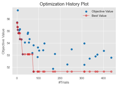
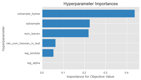
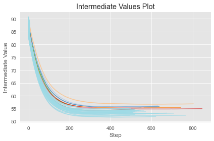
Using LGBMTuner from verstack - automated lightgbm models tuner with optuna (automated hyperparameter optimization framework).
Using Root Mean Squared Error as the metric for 500 trials.

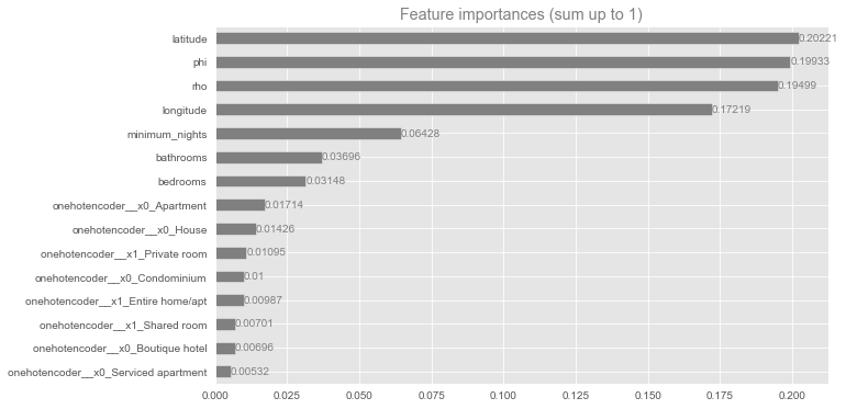
According to the tuned model:

• The most important hyperparameter is num_leaves: max number of leaves in one tree.

• The features with the most impact to the model are the geographic features phi, latitude, rho, longitude. Suggesting the location is a major factor in dictating price per night.

tuner = LGBMTuner(metric = 'rmse', trials = 500)
tuner.fit(X_train, y_train)

 * Initiating LGBMTuner.fit
     . Settings:
     .. Trying 500 trials
     .. Evaluation metric: rmse 
     .. Study direction: minimize rmse

     . Trial number: 0 finished
     .. Optimization score (lower-better): rmse: 55.67789244564906
 ...........................................................................
     . Trial number: 20 finished
     .. Optimization score (lower-better): rmse: 54.29340571492496
 ...........................................................................
     . Trial number: 55 finished
     .. Optimization score (lower-better): rmse: 54.05121505929641
 ...........................................................................
     . Trial number: 95 finished
     .. Optimization score (lower-better): rmse: 52.856645986642825
 ...........................................................................
     . Trial number: 175 finished
     .. Optimization score (lower-better): rmse: 53.08965433288682
 ...........................................................................

   - Tune n_estimators with early_stopping
Training until validation scores don't improve for 200 rounds
[100]	train's lgb_rmse: 57.4738	valid's lgb_rmse: 61.4568
[200]	train's lgb_rmse: 47.4023	valid's lgb_rmse: 56.3379
[300]	train's lgb_rmse: 42.7863	valid's lgb_rmse: 55.5581
[400]	train's lgb_rmse: 39.7538	valid's lgb_rmse: 55.6518
[500]	train's lgb_rmse: 37.4302	valid's lgb_rmse: 55.9252
Early stopping, best iteration is:
[344]	train's lgb_rmse: 41.314	valid's lgb_rmse: 55.5445

   - Fitting optimized model with the follwing params:
learning_rate                    : 0.01
num_leaves                       : 111
colsample_bytree                 : 0.705868674243541
subsample                        : 0.6737648484996459
verbosity                        : -1
random_state                     : 42
objective                        : regression
metric                           : rmse
num_threads                      : 14
reg_alpha                        : 1.830273189019251e-08
min_sum_hessian_in_leaf          : 0.0017813151887621482
reg_lambda                       : 0.0723651402085118
n_estimators                     : 344

     . Optuna hyperparameters optimization finished
     .. Best trial number:76    |     rmse:            51.64429482194801
 ---------------------------------------------------------------------------
     . n_estimators optimization finished
     .. best iteration:  344   |     rmse:             55.5445339314529
 ===========================================================================

Time elapsed for fit execution: 20 min 4.296 sec

# Best Performing Model
LGBMRegressor(**tuner.best_params)

LGBMRegressor(colsample_bytree=0.705868674243541, learning_rate=0.01,
              metric='rmse', min_sum_hessian_in_leaf=0.0017813151887621482,
              n_estimators=344, num_leaves=111, num_threads=14,
              objective='regression', random_state=42,
              reg_alpha=1.830273189019251e-08, reg_lambda=0.0723651402085118,
              subsample=0.6737648484996459, verbosity=-1)

y_pred = tuner.predict(X_test)
y_pred

array([149.52588627, 192.46170071, 239.86680096, ..., 225.76162168,
        96.80989254, 150.26631376])

Model Evaluation

Measure model performance using Mean Squared Error, Mean Absolute Error, Root Mean Squared Error, and r2 Score.

\[ MSE(y, \hat{y}) = \frac{1}{N_{samples}} \sum_{i=0}^{n_{samples} - 1} (y_i - \hat{y_i})^2 \]

\[ MAE(y, \hat{y}) = \frac{1}{N_{samples}} \sum_{i=0}^{n_{samples} - 1} | y_i - \hat{y_i} | \]

\[ R^2(y, \hat{y}) = 1 - \frac{\sum_{i=1}^{n} (y_i - \hat{y_i})^2}{\sum_{i=1}^{n} (y_i - \bar{y_i})^2} \]

Hyperparameter tuning improved the model’s RMSE from the base model.
Nevertheless, the RMSE scores is greater than 25 indicating that the model fails to predict price within 25 dollars off of the actual price.

performance_dict = {'MSE': mean_squared_error(y_test, y_pred), 
                    'RMSE': np.sqrt(mean_squared_error(y_test, y_pred)),
                    'MAE': mean_absolute_error(y_test, y_pred), 
                    'R2 Score': r2_score(y_test, y_pred)
                   }

performance_df = pd.DataFrame(performance_dict.items(), columns=['Metric', 'Score'])
performance_df

	Metric	Score
0	MSE	2899.750785
1	RMSE	53.849334
2	MAE	39.367336
3	R2 Score	0.612258

Outcome Summary

Aimed to predict price, allowing renters to estimate how much they could earn renting out their living space.
Adopted Supervised Machine Learning approach to predict labeled continuous target variable price using details about each property rented, as well as the price charged per night.
After model selection and tuning, the best model:

LGBMRegressor(colsample_bytree=0.6965557560964968, learning_rate=0.01,
              metric='rmse', min_sum_hessian_in_leaf=0.37294528370449115,
              n_estimators=314, num_leaves=142, num_threads=14,
              objective='regression', random_state=42,
              reg_alpha=6.532407584502388, reg_lambda=0.31928270201641645,
              subsample=0.5790593334642422, verbosity=-1)

The most important features of the model:

• geospaital features e.g.(phi, latitude, rho, longitude)
  Interesting considering price has the highest correlation with no. of bedrooms.

Resulting with a \(r^2\) Score of ~0.61 and ~53.75 RMSE. Though, failing to reach target of estimating prices that are less than 25 dollars off of the actual price.

Next steps

To improve the model and reach the target of estimating prices without being more than 25 dollars off:

• More data collection to increase training size.

• Record more features about the living space, e.g. amenities (parking, appliances, etc.), geographic features (nearby public transportation, etc.).

• Expand upon feature engineering and hyperparameter tuning.

• Use more complex models or ensemble methods, e.g. blending or stacking models.